Determining MP3 audio quality with spectral analysis

April 10, 2022

You might have an MP3 file that says it’s high quality, but you want to know for sure. Spectral analysis is a great method to determine the real bitrate, and thus the real quality, of an MP3 file. In this post, I explain a bit of theory regarding MP3 audio, and then I demonstrate how to analyze the spectrum of an audio file in practice and consequently deduce its bitrate.

Preliminary: a bit of theory

Before we start with the practical part, I’ll briefly cover some theoretical background to help you understand how the process works.

What is spectral analysis?

Essentially, it’s a way to analyse a sound in terms of its frequency spectrum, i.e. the individual frequencies that make up the sound. You take a sound file, and then run some calculations on it – for example, a Fast Fourier Transform is used pretty often. In any case, the end result is a graphical overview of the sound, showing which frequencies make up what you hear.

What’s the link between a frequency spectrum and audio quality?

That is, how does spectral analysis help you determine the quality of an MP3 file? Well, as you might know, MP3 files can be encoded at various bitrates. A file’s bitrate is the number of bits of information that it contains per second, and it’s measured in kilobits per second (kbps). So if the bitrate is higher, it contains more information per second, and vice versa. This translates to differences in sound quality: if there is more information per second (a higher bitrate), the quality of the sound is higher, because you have more frequencies per second and hence more detail. Some common bitrates for MP3 files are 128 kbps, 192 kbps, 256 kbps, and 320 kbps. As you can probably intuit, 128 kbps is the lowest quality, and 320 kbps is highest. The reduced information at lower bitrates translates to a smaller amount of frequencies per second, so MP3 encoders need a way to select which information to discard. This is solved with, among other things, a cutoff frequency: at lower MP3 bitrates, data above a certain threshold is discarded, and this threshold varies depending on the target bitrate. With spectral analysis, you can visually identify this threshold, and thus determine the bitrate.

As a side note: in this post, I will always be talking about constant bitrate files. If you have a 320 kbps file at constant bitrate, you always have 320 kilobits of information every second. You can also have a variable bitrate MP3, which has varying amounts of bits per second, and supposedly results in a smaller file size without a noticeable difference in quality.

But doesn’t an MP3 already tell you what bitrate it is?

With MP3 files, your music player will generally tell you the bitrate of the file. The problem is, this can be faked, so you might think you have a 320 kbps file, when it’s actually a 128 kbps file in disguise (see the practical part below, where we actually do this). If you transcode a file from 320 kbps down to 128 kbps, you’re losing information – approximately 192 bits of information per second (with some potential variability). You can also transcode a file from 128 kbps to 320 kbps, but you’ll still be at the sound quality of 128 kbps audio, because there’s no way to reconstruct those extra bits. You can’t just pull them out of thin air – once you go to a lower bitrate, there’s no way to get back the data that you lost in the process. So if you go the other way and transcode an MP3 from 128 kbps to 320 kbps, you’ll trick a music player into telling you that it’s high quality (because the file’s metadata will say that it’s 320 kbps audio), but the sound will still be the same. Fake high-quality MP3s are quite common particularly for audio that falls off a pirate ship.

Practical spectral analysis: uncovering the true bitrate of an MP3 file

This is where spectral analysis comes into the picture. Your music player might tell you that a sound file is high quality, but spectral analysis looks directly at the information in the audio file, so you’ll be able to tell immediately whether a file is genuinely high quality based on its cutoff frequency.

There are many tools for spectral analysis; I’ll be showing how to do this with SoX, a powerful command-line tool for audio processing. There’s also a way to do it with ffmpeg, but I’ve found SoX to be faster and with nicer output (plus it has many other uses). If you prefer graphical programs, you can use one of the Audacity forks like Tenacity or audacium – I won’t be covering that in this post, but search the internet for “plot spectrum” if you want to go the GUI route.

Setup: preparing some fake high-quality audio files

First, I’ll select an audio file that I made myself, let’s call it audio.flac. It’s in FLAC format, which is generally the highest possible quality you can obtain.

Next, I’ll use ffmpeg to transcode it to a high-quality 320 kbps MP3, and two different fake high-quality files at actual bitrates of 128 kbps and 256 kbps:

ffmpeg -i audio.flac -b:a 320k 320.mp3
ffmpeg -i audio.flac -b:a 256k temp.mp3 \
    && ffmpeg -i temp.mp3 -b:a 320k fake-at-256.mp3 \
    && rm temp.mp3
ffmpeg -i audio.flac -b:a 128k temp.mp3 \
    && ffmpeg -i temp.mp3 -b:a 320k fake-at-128.mp3 \
    && rm temp.mp3

Analyzing the files

With ffprobe (included with ffmpeg), we can check the supposed quality of these files:

for f in *.mp3; do printf "%s: %s\n" "$f" "$(ffprobe "$f" 2>&1 | grep Audio)"; done

This outputs:

320.mp3:   Stream #0:0: Audio: mp3, 44100 Hz, stereo, fltp, 320 kb/s
fake-at-128.mp3:   Stream #0:0: Audio: mp3, 44100 Hz, stereo, fltp, 320 kb/s
fake-at-256.mp3:   Stream #0:0: Audio: mp3, 44100 Hz, stereo, fltp, 320 kb/s

So all of these files are supposedly high quality, even though we know that’s not the case. Let’s see what spectral analysis tells us.

For each file, I’ll generate a spectrogram with sox:

sox audio.flac -n spectrogram -o flac.png -t FLAC
sox 320.mp3 -n spectrogram -o 320.png -t '320 kbps'
sox fake-at-256.mp3 -n spectrogram -o 256.png -t '256 kbps'
sox fake-at-128.mp3 -n spectrogram -o 128.png -t '128 kbps'

This yields the following four spectrograms (click the buttons to view):

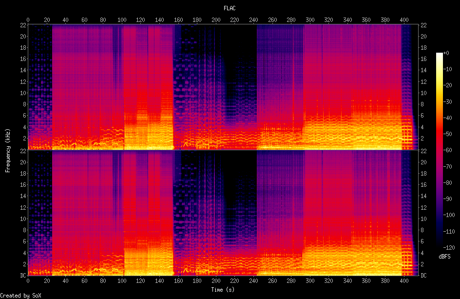
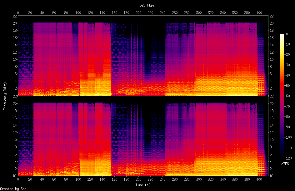
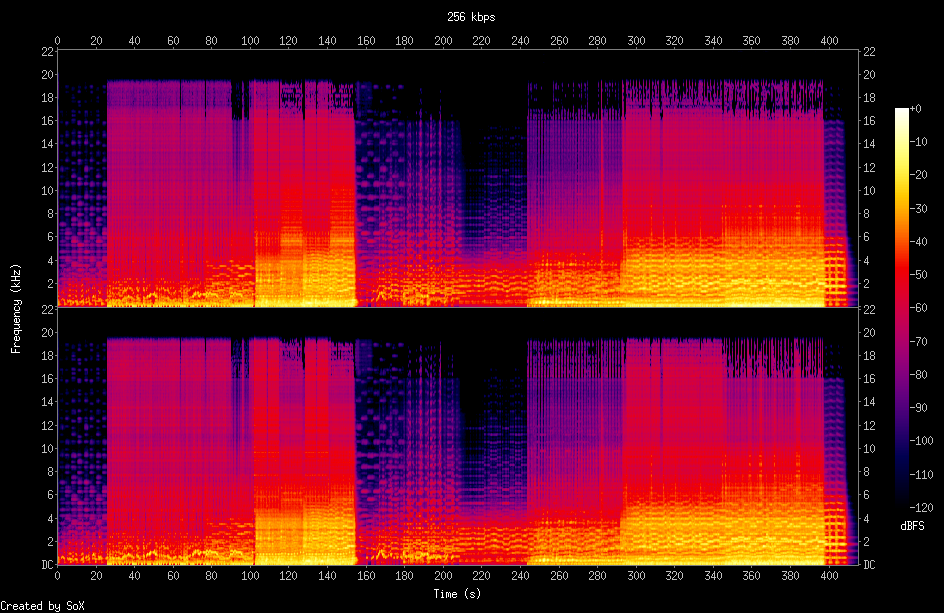
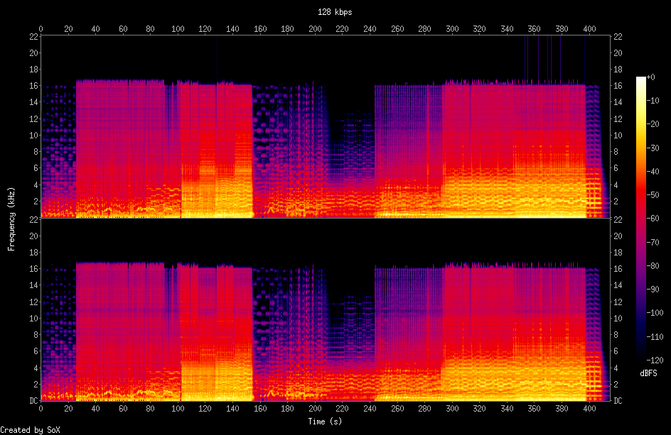
What you see in these images is a graphical overview of each of the audio files. In plain English, the plot shows you which frequencies are present in the audio at different points in time. The horizontal axis is time (i.e. the start of the audio is on the left, and the end is on the right). The vertical axis is the frequency, in kHz, and the colors show the amplitude of each frequency at different points in time. Since this audio is in stereo, the top subplot shows the left audio channel, and the bottom subplot shows the right audio channel.

So, how can you use this information? Well, an important observation is that there is a cutoff frequency, a ‘threshold’. If you compare the FLAC audio to the 320 kbps audio, you’ll notice that the 320 kbps audio does not have any data past the 20 kHz mark on the vertical axis, where the FLAC audio has frequencies up to 22 kHz (for example starting at around 25 seconds and around 243 seconds on the horizontal axis). If you then go to lower quality files, you’ll notice that the cutoff threshold decreases: at 256 kbps it’s around 19 kHz, and at 128 kbps it’s at around 17 kHz. Comparing these plots, you can see exactly how much less data (and hence sound detail) you end up with at lower bitrates. You can also see how much data you lose when converting from FLAC to 320 kbps (though whether this makes any practical difference when listening to audio varies by person; the consensus is that humans hear up to 20 kHz, so 320 kbps MP3 should be fine, but some swear by only FLAC files, and it might actually matter if you have high-quality audio equipment – unfortunately I don’t).

Based on these graphs, we can see that while all of the MP3 files were pretending to be high-quality, only one of them really is – the one with a cutoff frequency of around 20 kHz. The rest are just pretenders and fakes.

Conclusion

In summary, this post introduced a bit of theory about MP3 audio, and practically demonstrated spectral analysis of MP3 files. Next time, if you’re uncertain about the quality of an MP3 file, just run sox and if the spectrum shows a cutoff below 20 kHz, the file is probably not encoded at 320 kbps.

PS: Since you read this far, I’ll share a trick that I use and that works decently well most of the time: estimating the file size and comparing the estimate with the actual file size. At 320 kbps (kilo bits per second), you’ll have 40 KB (kilo bytes per second), because there are 8 bits in a byte and 320 / 8 = 40. So per minute, you’ll have 2400 KB, or 2.4 MB. Let’s say you have an MP3 file with an audio length of 3:27. That’s approximately 3.5 minutes. Then you do a quick calculation: 3.5 minutes × 2.4 MB/minute = 8.4 MB. So if you look at the total file size, it should be around 8.4 MB. If it’s significantly less than that, you’re probably looking at a lower quality MP3 file. This method might not always work, but it’s a nice additional check that you can do. If you’re uncertain, spectral analysis is the best approach.